Examples
Performing Traces
Setting up Initial Conditions
Initial conditions are configured using the ParticleState class. In the below example, we setup one particle starting at (-6.6, 0, 0) Earth Radii. To configure multiple particles, arrays of longer length can be provided.
Because DISCO uses the mass and charge of the particles to dimensionalize the simulation, it can only do traces for one combination of mass and charge at a time. Unless otherwise specified, all coordinates used in DISCO are Solar Magnetic (SM).
import disco
from astropy import constants, units
import numpy as np

particle_state = disco.ParticleState(
    x = np.array([-6.6]) * constants.R_earth,
    y = np.array([0.0]) * constants.R_earth,
    z = np.array([0.0]) * constants.R_earth,
    ppar = np.array([0.8]) * constants.m_e * constants.c,
    magnetic_moment = np.array([800]) * units.MeV / units.G,
    mass = constants.m_e,
    charge = constants.e.si,
)
Setting Magnetic and Electric Field Models
Traces can be performed in magnetic and electric field context loaded from output of MHD simulations or taken directly from user-provided arrays.
Currently, loading output from the Space Weather Modeling Framework (SWMF) is built-in, with future plans to add support for MAGE. To load from the output of MHD simulations, we use the disco.readers module. Below is an example loading from SWMF.
import disco
from disco.readers import SwmfOutFieldModelDataset

dataset = SwmfOutFieldModelDataset('swmf_run/*.out')

field_model_loader = disco.DynamicFieldModelLoader(
   dataset, config, particle_state.mass, particle_state.charge
)
To directly provide the fields in arrays, the following snippet can be used. The magnetic field is expected to be the external magnetic field, i.e. with the dipole subtracted. The strength of the dipole used during interpolation can be configured with the B0 keyword argument.
import disco
from astropy import constants, units
import numpy as np

# Setup axes for the field model
grid_spacing = 0.1
x_axis = np.arange(-10, 10, grid_spacing) * constants.R_earth
y_axis = np.arange(-10, 10, grid_spacing) * constants.R_earth
z_axis = np.arange(-5, 5, grid_spacing) * constants.R_earth
t_axis = np.array([0, 60]) * units.s

x_grid, y_grid, z_grid, t_grid = np.meshgrid(
    x_axis, y_axis, z_axis, t_axis, indexing="ij"
)

r_inner = 1 * constants.R_earth

axes = disco.Axes(x_axis, y_axis, z_axis, t_axis, r_inner)

# Setup field model (zero external field --> dipole)
Bx = np.zeros(x_grid.shape) * units.nT
By = np.zeros(Bx.shape) * units.nT
Bz = np.zeros(Bx.shape) * units.nT
Ex = np.zeros(Bx.shape) * units.mV / units.m
Ey = np.zeros(Bx.shape) * units.mV / units.m
Ez = np.zeros(Bx.shape) * units.mV / units.m

field_model = disco.FieldModel(Bx, By, Bz, Ex, Ey, Ez, axes)
DISCO requires at least two timesteps of field model context so that it can interpolate in both space and time. If you only have one timestep, use the duplicate_in_time() method to synthetically copy it to two timesteps.
import disco

field_model = disco.FieldModel(Bx, By, Bz, Ex, Ey, Ez, axes)
field_model = field_model.duplicate_in_time()
Starting the Trace
The last thing to setup is the disco.TraceConfig object, which controls configuration options for trace. To do a trace between two times, we can specify the t_initial and t_final parameters.
An important parameters for disco.TraceConfig is output_freq, which controls how often the trace will output results. By default, only the first and last timesteps are outputted, so if you want to output every timestep, you need to set output_freq=1.
import disco
from astropy import units

config = disco.TraceConfig(
    t_initial = 0 * units.s,
    t_final = 30 * units.s,
    output_freq = 1,  # Output every timestep
)
Now we can perform the trace using disco.trace_trajectory(). This function takes the config, particle_state, and field_model_loader as arguments, and returns a disco.ParticleHistory object that contains the results of the trace. If you created a disco.FieldModel directly from arrays, you can pass it instead of field_model_loader.
import disco

history = disco.trace_trajectory(
    config, particle_state, field_model_loader
)
How that you have a history object, you can move on to the next section to save it or plot it.
Saving and Plotting Results
Saving and Loading from Disk
When a trace is performed with disco.trace_trajectory(), it returns an instance of disco.ParticleHistory. This object can be saved to an HDF5 file using the history.save() method:
import disco

history = disco.trace_trajectory(
   config, particle_state, field_model_loader
)

history.save('DiscoTrajectoryOutput.h5')
Later on, the object can be restored from this HDF5 file using the disco.ParticleHistory.load() method:
history = disco.ParticleHistory.load('DiscoTrajectoryOutput.h5')
Built-in Plotting Methods
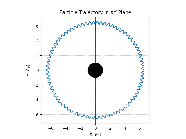
The disco.ParticleHistory object has built-in plotting methods to visualize the results of the trace. The history.plot_xy() method plots the trajectory in the XY plane, while plot_xz() and plot_yz() plot the trajectory in the XZ and YZ planes, respectively. These methods can be passed a matplotlib axes object to plot on, or they will create a new figure and axes if none is provided.
import disco
from matplotlib import pyplot as plt

history.plot_xy()  # Plot trajectory in XY plane
plt.savefig('trajectory_xy.png')
The plotting methods also support the inds= keyword argument, which allows you to plot only a subset of the particles in the history. For example, to plot only the first particle, you can do:
# Plot only the first particle in XY plane
history.plot_xy(inds=[0])
Also supported is a sample= keyword argument, which allows you to plot only random sample of the particles traces. For examples, to plot a random sample of 1,000 particles, you can do:
# Plot a random sample of 1,000 particles in XY plane
history.plot_xy(sample=1000)
Advanced Options
Backwards-Time Integration
Backwards time integration can be done by passing integrate_backwards=True to disco.TraceConfig. When this is done, the value of t_final should be less than t_initial. The value of the default step size, h_initial, should always be positive.
import disco
from astropy import units

config = disco.TraceConfig(
    t_initial = 0 * units.s,
    t_final = -30 * units.s,
    integrate_backwards=True,
)
Tracing in non-Time-Dependent Fields
DISCO requires at least two timesteps of field model context so that it can interpolate in both space and time.
If you are loading from simulation output, index the dataset at the desired timestep position and call the duplicate_in_time() function to create a disco.FieldModel which you can pass to disco.trace_trajectory().
from disco.readers import SwmfOutFieldModelDataset

dataset = SwmfOutFieldModelDataset('swmf_run/*.out')
field_model = dataset[0].duplicate_in_time()
If you are directly providing arrays for the magnetic and electric field context, simply call duplicate_in_time() on the disco.FieldModel instance.
import disco

field_model = disco.FieldModel(Bx, By, Bz, Ex, Ey, Ez, axes)
field_model = field_model.duplicate_in_time()
Loading from Custom Simulation Output
For ambitious users who want to support dynamic loading of non-built-in magnetic and electric field models, this can be done by authoring a subclass of disco.readers.FieldModelDataset. The user will need to implement the following methods:
__len__(self): returns the number of timesteps in the dataset__getitem__(self, index): returns adisco.FieldModelinstance, with a single timestep, for the given timestep index. TheAxesused to create thisFieldModelshould have the single timesteptvalue set correctly.get_time_axis(self): returns an array with units of time, of size equal to the number of timesteps, that describes the timestamps of each index
When that subclass is implemented and working, it can be used with disco.DynamicFieldModelLoader, which will call __getitem__ on demand as new timesteps are needed. This instance of disco.DynamicFieldModelLoader can be passed to disco.trace_trajectory to cause the trace to use your output.
import disco

dataset = MyDataset("some_directory/*.cdf")

field_model_loader = disco.DynamicFieldModelLoader(
    dataset, config, particle_state.mass, particle_state.charge
)